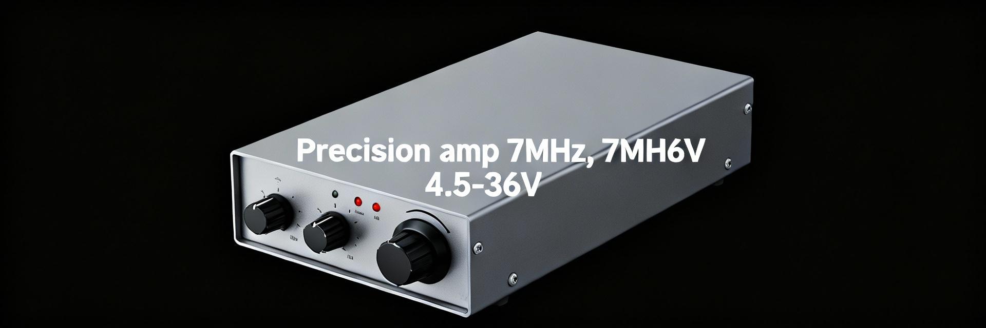
Point: A data-driven snapshot frames expectations for this mid‑GBW precision amplifier. Evidence: Typical device numbers include a GBW around 7 MHz, supply voltage range ≈ 4.5–36 V, slew rate near 20 V/µs, input offset in the tens–low hundreds of µV, and output drive up to ~32 mA per channel. Explanation: These specs position the amplifier for precision sensor buffers and mid‑frequency analog front ends where supply flexibility and moderate bandwidth are required.

TP1282L1-VR: Quick Specs Overview (Background)

Key electrical specs at a glance

Point: Headline specs summarize capability and limits. Evidence: GBW ≈ 7 MHz; supply voltage 4.5–36 V; typical quiescent current per channel in the low mA range; input offset tens–hundreds of µV typical; slew rate ≈ 20 V/µs; output current up to ~32 mA; input common‑mode and output‑to‑rail behavior show limited rail‑to‑rail margins. Explanation: Knowing typical versus absolute‑max values helps set expectations for drift, load driving, and achievable closed‑loop bandwidth in real circuits.

How to read these datasheet values (what's conservative vs. typical)

Point: Typical numbers are measured under specific lab conditions; maximum/minimum guarantees include margins. Evidence: Datasheet "typical" columns usually reflect 25°C, specified test circuit, and single unit examples, while "max/min" values are production limits across temperature. Explanation: On real PCBs offset, quiescent current (Iq), and output swing vary with temperature, supply headroom, and layout; designers should budget the worst‑case (max/min) for critical analog chains.

Detailed GBW & Frequency Performance (Data analysis)

What GBW = 7 MHz means for closed-loop gain and bandwidth

Point: GBW governs closed‑loop bandwidth per the rule of thumb. Evidence: Closed‑loop bandwidth ≈ GBW / closed‑loop gain, so at GBW=7 MHz the -3 dB points are roughly: gain=1 → 7 MHz, gain=2 → 3.5 MHz, gain=10 → 700 kHz. Explanation: This directly affects sensor buffers, anti‑alias filters and active integrators — choose closed‑loop gain with the desired passband margin and allow headroom for phase margin and component tolerances.

Slew rate, phase margin, and large-signal behavior

Point: Slew rate limits large‑signal slew and impacts transient distortion. Evidence: With slew ≈ 20 V/µs, a 10 Vpp fast edge requires ≈ 0.5 µs to slew from peak to peak, adding settling delay and potential slew‑induced distortion at high amplitude/frequency. Explanation: For aggressive feedback or high‑amplitude signals use lower closed‑loop gains, add compensation where needed, and bench verify large‑signal settling and THD to ensure the amplifier meets system requirements.

TP1282L1-VR Voltage & Power Deep-Dive (Method / Data)

Supply voltage range and headroom (supply voltage, input/output swing)

Point: Wide supply range enables single‑supply and high‑voltage applications. Evidence: Operating from about 4.5 V to 36 V allows single‑supply use at 5–12 V or split rails ±6–±18 V, but input common‑mode and output swing do not reach rails; expect several hundred millivolts to a volt of headroom depending on load. Explanation: Designers must verify input common‑mode windows for sensor interface and anticipate degraded swing under heavier loads; level shifting or rail‑to‑rail parts are needed when true rail reach is required.

Quiescent current, output drive and thermal/power dissipation

Point: Power dissipation combines Iq and dynamic output losses. Evidence: Pd ≈ Vsup × Iq + dynamic losses from driving RL; example: with Iq ≈ 1.2 mA/channel at 36 V, static Pd ≈ 43 mW per channel, plus AC losses when sourcing 32 mA into loads. Explanation: For high supply voltages or continuous high‑current drive compute junction rise, allocate copper area, and derate device if ambient or package limits are approached to avoid thermal drift or damage.

Measurement Methods & Bench Test Setup (Methods / How-to)

How to measure GBW and slew rate — step-by-step

Point: Repeatable test procedures yield reliable GBW and slew numbers. Evidence: Use a network analyzer or function generator + scope: configure closed‑loop gain of 1 and 10, apply small‑signal sine sweep for Bode plot, record -3 dB cutoff to infer GBW; for slew apply a large amplitude step (e.g., 2–5 V step) and measure dV/dt on the output. Explanation: Capture probe loading, scope bandwidth, and test‑circuit capacitance in notes; report both small‑signal GBW and large‑signal slew behavior since they determine different aspects of real performance.

Supply-voltage stress tests and input/common-mode checks

Point: Verify operation across the full supply envelope. Evidence: Test at low end (≈4.5 V), typical mid points (e.g., 12 V), and high end (≈36 V): monitor offset, drift, output swing, and distortion while exercising representative loads. Explanation: Include decoupling, series protection, and limit current during initial evaluations; document behavior near common‑mode limits and watch for increased offset or reduced output swing at extremes.

Real-world Use Cases & Performance Examples (Case study)

Example: sensor buffer and single-supply operation (5–12 V)

Point: Practical sensor interface design uses GBW and offset budgets. Evidence: For a unity or gain‑of‑2 buffer for a sensor with 100 kHz content, GBW=7 MHz yields ample margin (bandwidths of 7 MHz and 3.5 MHz respectively), while offset in the tens of µV keeps low‑frequency error minimal. Explanation: Add input filtering, choose feedback resistors to control noise, and implement offset trim or digital calibration when absolute accuracy matters.

Example: higher-voltage buffer (±12 V rails) and driving loads

Point: High‑voltage rails expand headroom but increase dissipation. Evidence: Driving a 2 kΩ load with ±12 V rails and output swing ±10 V draws up to 5 mA; static Pd from Iq plus dynamic losses can approach package limits if multiple channels are active. Explanation: Compute thermal margin, keep copper under the package generous, and assess settling time — slew and load interaction will lengthen settling for large steps.

Design Checklist & Recommendations for Engineers (Action)

PCB, decoupling and layout best practices

Point: Layout directly affects stability and noise. Evidence: Use local decoupling (0.1 µF ceramic + 10 µF bulk close to pins), short ground returns, guard traces for sensitive inputs, and thermal copper pads beneath the package. Explanation: Good layout minimizes supply bounce, preserves phase margin, and reduces offset drift; document decoupling values and placement in the BOM and PCB notes.

Specification tradeoffs and when to choose alternatives

Point: Match application priorities to amplifier tradeoffs. Evidence: If GBW or slew are the dominant limits choose a higher‑GBW device; if offset dominates precision choose a lower‑offset, lower‑noise amp; for battery operation prioritize low Iq. Explanation: Establish pass/fail criteria (bandwidth, offset, noise, power) early; bench test alternatives with identical circuits to compare system‑level impact before lock‑in.

Conclusion

Point: Practical takeaways guide integration and test. Evidence: The amplifier’s mid‑GBW (~7 MHz), broad supply range (~4.5–36 V), ~20 V/µs slew rate, low µV‑level offsets, and ~32 mA drive make it suitable for precision sensor buffers and analog front ends with modest bandwidth needs. Explanation: Verify closed‑loop bandwidth vs. GBW, perform supply‑extreme tests, and follow PCB/layout and thermal guidance to ensure reliable field performance.

Key Summary

• Understand GBW: closed‑loop bandwidth ≈ 7 MHz / gain; plan for gain=1→7 MHz, gain=10→~700 kHz.
• Mind supply headroom: 4.5–36 V enables many modes but expect limited rail swing under load.
• Test for real behavior: measure GBW, slew, offset and thermal dissipation across supply extremes and loads.
• Layout matters: local decoupling, short returns, and thermal copper are required for stable, low‑noise operation.

Common Questions and Answers

How should engineers measure GBW for this amplifier?

Use a network analyzer or a function generator and scope with a closed‑loop test circuit (gain=1 and gain=10). Sweep a small‑signal sine and note the -3 dB cutoff; multiply cutoff by closed‑loop gain to verify GBW. Document probe loading, test amplitude, and temperature for repeatable results.

What supply tests reveal the most about real-world performance?

Run tests at the low, mid, and high supply extremes (≈4.5 V, a mid value like 12 V, and ≈36 V) while measuring offset, drift, output swing under load, and distortion. Include thermal monitoring and decoupling to capture realistic behavior under expected operating conditions.

When is the slew rate likely to limit system performance?

If your application uses large amplitude, high‑frequency transients (for example, >5 V steps or high‑frequency AC near the closed‑loop bandwidth), the ~20 V/µs slew will slow edges and increase settling time; verify with time‑domain step tests and consider a higher‑slew amplifier if needed.